Messages

[To me, that's the hardest part(and tempo will also be taken into account).]

Actually I already have a basic draft on implementing OODA AI in RPGs using the default battle system(those in RMVXA, RMMV, etc), charge turn battle and active time battle.

Basically, implementing the observe section will be defining what can be observed under what conditions. The AI should be able to observe almost everything from the allies, but only limited information from the opponents.

Implementing the orient section will need a knowledge database - list of strategies and list of tactics, a memory storing past events in battles, and the result of the observation.
Then fuzzy logic can be used to give a rating on how much the current situation, combined with past experiences, manifests those strategies and tactics.
After that, fuzzy logic can also be applied to give a rating on how excellent a strategy/tactic(building block strategy/tactics or composite ones based on those building blocks) can counter the estimated strategies/counters executed by opponents. To me, that's the hardest part(and tempo will also be taken into account).

Implementing the decide section will be based on the rating for each strategy/tactic countering the opponent's ones.
For instance, the AI can simply randomly pick 1 among the 5 strategies/tactics with the highest rating.

Implementing the act section will be based on the decided strategy/tactic. The AI should be able to turn a general strategy/tactics into concrete action plans, according to what the AI has observed.
From all currently available moves(including doing nothing), the AI should be able to give a rating on how much each move can contribute to the decided strategy/tactic.
To me, that's the second hardest part, especially in real time battle systems(mainly because of time performance issue).

I can already foresee that, the OODA AI implementation will be heavily based on the strategy pattern.

P.S.: I think that state machines will suffice for small scale OODA AIs facing low complexities, but they'll probably fail in large scale complex use cases.

[oversimplified]

First, let's cite what OODA is:
- OODA loop
- The Tao of Boyd: How to master the OODA Loop
- Unlocking the power of Colonel John Boyd's OODA Loop

After reading all those, you, as a game developer, might wonder: How can we use OODA to write battler AI? Let's start with exploring the following oversimplified version:
(The below assumes that the battler AI are built to minimize the chance for the players to win. The OODA will be used slightly differently if that's not the battler AI's ultimate goal.)

Observe
To observe is to receive as many relevant info as accurately(including fake info detections by verifications) as possible. However, what can be observed by a battler?
(For the sake of writing battler AI, issues with fake info can be safely ignored as all relevant info can always be accurately received by any RMVXA battler AI.)
I think that any normal battler should be able to observe the opponents' current party/troop formations(like consisting of which actors/enemies), all their executed actions, and the allies' current statuses(like having which states/buffs/debuffs and how many hp/mp/tp).
Sometimes it could, however, be unfair for a battler to be able to observe the opponents' current capabilities(like classes, equips, parameters, extra parameters, special parameters, level and skill lists) or carried items.

For example, at the start of a battle, a boss facing a 6 actor party might be able to observe that all those actors are:
- heavily geared towards dealing damage with significant sacrifice from every other battle aspect, and/or
- mages only excelling at using magics, and/or
- fighters only excelling at using physical moves, and/or
- totally unresistant to some states/debuffs, and/or
- drastically faster than that boss(in action battle system, active time battle, charge turn battle, tactical battle system, etc), and/or something else.

Orient
To orient is to use mental models to make sense of those observed info(including judging the underlying implications and meanings) to fathom the current situations to generate working action plans. This process are affected by the following factors:
(For the sake of battler AI, mental models means the complete frameworks consisting of all the known strategies and tactics with all their known counters in the addressed RMVXA games that can be used by the allies, opponents and the battlers themselves.)
- New Information
- Previous Experience
- Cultural Traditions
- Genetic Heritage
- Analysis and Synthesis
For the sake of writing battler AI, cultural traditions and genetic heritage can be regarded as a battler's characters if they've to be taken info account, or simply ignored if they don't.
About the rest:
- New information must always be taken into account. Otherwise the battler AI will fail to realize that the situations have changed, let alone adapting to them(or better yet, controlling them).
- Previous experience, which will be fed by the new information, must always be taken into account too. In terms of battler AI, it means the AI will have to store all the relevant info in the current battle so far. Sometimes the full pictures, like the opponents' strategies, can only be accurately formed by combining the previous experience with the new information.
- Analysis means breaking down the existing mental models into smaller pieces, while synthesis means using those smaller pieces to form new mental models that can accurately address the new situations. This implies that the battler AI should be written to include as many known strategies and tactics with as many of their counters as possible, and they should all be able to be broken down into independent modular pieces that can be integrated into new strategies and tactics with their own counters. It also means that the battler AI should be able to judge which pieces are called for and run the integrated strategies and tactics by combining all those pieces.

For example:
- At the start of a battle, a boss fighting a 6 actor party observed that they're all heavily geared towards dealing damage with significant sacrifice from every other battle aspect.
By recalling all the known strategies and tactics with their counters, the boss AI will realize that it's extremely likely that that 6 actor party will try to kill the boss as quickly as possible(strategies) by having as high damage throughput as possible(tactics).
The boss AI will then use all the known strategies and tactics to generate all the ones that can counter the players' ones.
- In action battle system, active time battle, charge turn battle, tactical battle system, or any other battle system having the time dimension, a boss noticed that some actors just halted momentarily even when they should have acted instead(whether they should act instead needs orientations to tell) in some situations.
The boss AI will know that it's highly probable that the players aren't good at addressing those situations yet.
The boss AI will then use all the known strategies and tactics to generate all the ones that can make those situations happen more frequently.

Orientation's the most important part as it determines how accurate the observations will be interpreted and how useful the generated solutions will be executed.
For the sake of the battler AI, orientation's also the hardest part to be implemented well as it needs to stores all the known strategies and tactics with all their known counters, and the algorithms decoding the opponents' ones and coming up with all the working counters.

Decide
To decide is to judge which of all the generated action plans will be the best calls for the addressed situations which are already accurately fathomed. All these judgments should be treated as the best hypothesis which are to be tested rather than absolutely correct choices.

For example:
- At the start of a battle, a boss fighting a 6 actor party figured out that the party tried to kill the boss as quickly as possible(strategies) by having as high damage throughput as possible(tactics), and the boss AI has already generated all counters that can work.
The boss AI then forms the hypothesis that "it's better to mix several counters together to confuse the players by obfuscating the intentions" and decided to build action plans around that.

Act
To act is to build the action plans around the decisions and test those action plans by executing them(either simultaneously or treating the rest as backups that can always be quickly called). Then observations will be needed to check if those action plans worked and which ones work the best(and they'll be the main ones until the new best comes) in order to "finish"(and then restart) the "infinite" loop.

For example:
- A boss executes several counters together in a mixed manner to stop the players' strategies and tactics.
As the players realized they've been countered, they begin to adapt and use new strategies and tactics instead.
The boss AI noticed that the players are adapting to the new situations so the boss reorient in order to form new hypothesis to build and execute new action plans that will work.

Tempo
When it comes to oppositions, the faster one can effectively and efficiently run the OODA loop(higher velocity) and the faster one can change its tempo(higher acceleration), the more advantageous one will usually be in general. By controlling that tempo well via changing it rapidly and surprisingly, it's even possible to get inside the others' OODA loops to consistently reset them to the observe phase so they'll be confused and have to passively react to the new situations(they'll eventually end up being paralyzed in observations or making rash actions that won't work at all), while the one gaining the upper hand can constantly have an accurate full pictures and active control to the new situations.

For example:
- At the start of a battle(In action battle system, active time battle, charge turn battle, tactical battle system, or any other battle system having the time dimension) having 2 bosses, they act whenever they become able to by making moves that don't need charging(time delay between attempting to make a move and actually making that move).
This possibly led to players think that "act whenever becoming able to" are those bosses' patterns and those players build their action plans around their hypothesis.
Then suddenly those bosses delayed for a long time even when they become able to act, and that potentially lures players into thinking that those bosses are trying to make moves with long charging times so they make moves(which need to charge) that can cancel opponents' charging moves.
But that's exactly what those bosses want the players to do so instead those bosses make some other moves that don't need charging when the players are charging their moves.
The players now become confused and have to observe the new situations to form new mental models that can accurately address the new situations, while those bosses can take advantage from the resets of the players' OODA loops.

Building such battler AI won't be easy nor simple even for AI professionals. The builders need to have a thorough understanding to the battle systems, the battles and all the possible battlers involved as well as a fluent command on programming AI in general. Nevertheless, I still think that such AI would be incredibly challenging and extraordinarily difficult to beat if it could ever be built.

P.S.: Bear in mind that the aforementioned are still just an oversimplified version of the original OODA, which would certainly be overkill in writing battler AI.

[Points]

I'm only going to cover simple shapes like Points, Straight Lines, Circular Arcs, Circular Sectors and Simple Polygons, by using cartesian coordinates, basic algebra and Euclidean 2D geometry only. More complex shapes like ellipse and parabolas won't be covered, and more advanced maths like polar coordinates and affine spaces won't be used. No solid proofs will be covered as well. The below aims to always ensure 100% correctness, even for the teleportation cases, although it indeed fails a bit and badly when few and many shapes move quickly respectively.

Points
It's just an ordered x, y pair in the cartesian coordinate system.

Straight Lines
It's just the line between 2 specified points. The line will be represented by its corresponding linear equation in the form of y = mx + c. The rotation and translation offsets, valid x and y ranges and midpoint of the straight line will be used as well.
Users only has to define those 2 specified points. The rest will be generated by scripts upon initializing the point.

Circular Arcs
A virtual circular sector will be used to implement a circular arc, which is the real shape. Check below for Circular Sectors. The midpoint is used in the circular arc as well.

Circular Sectors
It's a system of 3 inequalities in 2 unknowns, including 2 linear ones in the form of y >= mx + c, y > mx+ c, y <= mx+ c or y < mx+ c, and 1 inequality of circle in the form of (x - h) ^ 2 + (y - k) ^ 2 <= r ^ 2 or (x - h) ^ 2 + (y - k) ^ 2 < r ^ 2. The center, radius, rotation and translation offsets, and associated equations for those inequalities will be used as well. Note that the center is also the intersecting point of those 2 linear inequalities.
Users only has to define the center, radius, and those 2 linear inequalities. The rest will be generated by scripts upon initializing the circular sector.

Simple Polygons
It's a system of linear inequalities in 2 unknowns. The number of inequalities is that of the edges. The vertexes, triangles of the polygon touching its edges and their incenters, an arbitrary center inside the polygon, the associated linear equations for those linear inequalities with their valid x and y ranges, the rotation and translation offsets, and the bounding rectangle or circular sector and inner circular sector or rectangle(analogous to inner circle) are used as well.
Users only has to define the vertexes, an arbitrary center inside the polygon, and whether a rectangle or circular sector will be used to bound the simple polygon. The rest will be generated by scripts upon initializing the simple polygon.

There are 5(5 + 1) / 2 = 15 possible cases: Points vs Points, Points vs Straight Lines, Points vs Circular Arcs, Points vs Circular Sectors, Points vs Simple Polygons, Straight Lines vs Straight Lines, Straight Lines vs Circular Arcs, Straight Lines vs Circular Sectors, Straight Lines vs Simple Polygons, Circular Arcs vs Circular Arcs, Circular Arcs vs Circular Sectors, Circular Arcs vs Simple Polygons, Circular Sectors vs Circular Sectors, Circular Sectors vs Simple Polygons, and Simple Polygons vs Simple Polygons.
For all cases, the collision flag and relative positions between 2 shapes will be stored upon change per frame. If the relative positions between 2 shapes remains unchanged, it's certain that their collision flag doesn't need to change and can be used directly. The time complexity here's O(1).

Points vs Points
Just compare if they have both the same x and y coordinates. The time complexity's O(1).

Points vs Straight Lines
The point's reference point will be adjusted to be that of the straight line. The time complexity here's O(1).
Then just check if the point's x and y coordinates are within the valid ranges of those of the straight line, and if that point's an solution to that linear equation. The time complexity here's O(1).
The combined time complexity's O(1).

Points vs Circular Arcs
The point's reference point will be adjusted to be that of the circular arc. The time complexity here's O(1).
Then just check if the distance between the point and the virtual center of the circular arc equals to the virtual radius of that circular arc, and if that point satisfies the 2 virtual linear inequalities in 2 unknowns.The time complexity here's O(1).
The combined time complexity's O(1).

Points vs Circular Sectors
Same as Points vs Circular Arcs, except that whether the distance between the point and the center is less than or equal to, or less than, the radius is checked instead of checking against the equal condition.

Points vs Simple Polygons
The point's reference point will be adjusted to be that of the simple polygon. The time complexity here's O(1).
The point will first the checked against the bounded rectangle or circular sector of the simple polygon. Checking a point against a circular sector goes to Points vs Circular Sectors, and that against a rectangle will be checking if both the x and y coordinates of the point lines between the minimum and maximum x and y coordinates of the rectangle. The time complexity here's O(1).
If the point doesn't collide with the bounded rectangle or circular sector of the simple polygon, then that point isn't colliding with that simple polygon itself. The combined time complexity will be O(1).
If that's not the case, then check the point against the inner rectangle or circular sector of the simple polygon, which is essentially the same as checking against the bounding ones.
If the point collides with the inner rectangle or circular sector of the simple polygon, then so does the simple polygon. The combined time complexity will be O(1).
If that's not the case, then check if the point satisfies all the linear inequalities of the simple polygon. The time complexity here's O(E), where E is the number of edges.
The combined time complexity will be O(E) in this case.

Straight Lines vs Straight Lines
Either straight line's reference point will be adjusted to be that of the other. The time complexity here's O(1).
Then just check if the 2 linear equations has solutions and whether the they lie within the valid ranges of both straight lines. The time complexity here's O(1).
The combined time complexity's O(1).


Straight Lines vs Circular Arcs
The straight line's reference point will be adjusted to be that of the circular arc. The time complexity here's O(1).
Then just check if the linear equation and the equation of circle has solutions and whether they satisfy the valid ranges of the straight line, and the 2 linear inequalities of the circular arc. The time complexity here's O(1).

Straight Lines vs Circular Sectors
The straight line's reference point will be adjusted to be that of the circular sector. The time complexity here's O(1).
The midpoint of the straight line will be checked against the circular sector. Checking a point against a circular sector goes to Points vs Circular Sectors. The time complexity here's O(1).
If the midpoint collides with the circular sector, then so does the straight line. The combined time complexity will be O(1).
If that's not the case, then it's certain that the straight line won't completely lie within the circular sector, meaning the former must intersect with the perimeter of the latter in order to collide. So checking whether the straight line collides with the linear equations or equation of circle of the circular sector will suffice.
They go to Straight Lines vs Straight Lines and Straight Lines vs Circular Arcs. The time complexity here's O(1).
The combined time complexity will be O(1) in this case.

Straight Lines vs Simple Polygons
The straight line's reference point will be adjusted to be that of the simple polygon. The time complexity here's O(1).
The straight line will be checked against the bounded rectangle or circular sector of the simple polygon. Checking a straight line against a circular sector goes to Straight Lines vs Circular Sectors.
That against a rectangle will be checking the midpoint of the straight line against that rectangle. Checking a point against a simple polygon goes to Points vs Simple Polygons.
If the midpoint collides with the rectangle, then so does the straight line. The time complexity will be O(1) but not O(E), as the number of edges of a rectangle's always 4.
If that's not the case, then it's certain that the straight line won't completely lie within the rectangle, meaning the former must intersect with the perimeter of the latter in order to collide. So checking whether the straight line collides with the linear equations of the rectangle will suffice.
It goes to Straight Lines vs Straight Lines. The time complexity here's O(1).
If the straight line doesn't collide with the bounded rectangle or circular sector, then neither does the simple polygon. The combined time complexity will be O(1).
If that's not the case, then check the straight line against the inner rectangle or circular sector of the simple polygon, which is essentially the same as checking against the bounding ones.
If the straight line collides with the inner rectangle or circular sector of the simple polygon, then so does the simple polygon. The combined time complexity will be O(1).
If that's not the case, then check the midpoint of the straight line against the simple polygon. Checking a point against a simple polygon goes to Points vs Simple Polygons.
If the midpoint collides with the simple polygon, then so does the straight line. The combined time complexity will be O(E).
If that's not the case, then it's certain that the straight line won't completely lie within the simple polygon, meaning the former must intersect with the perimeter of the latter in order to collide. So checking whether the straight line collides with the linear equations of the simple polygon will suffice.
It goes to Straight Lines vs Straight Lines. The time complexity here's O(E) but not O(1), as E instead of 1 straight lines have to be checked against.
The combined time complexity will be O(E) in this case.

Circular Arcs vs Circular Arcs
Either circular arc's reference point will be adjusted to be that of the other. The time complexity here's O(1).
Then just check if the equation of circles has solutions and whether they satisfy all the 4 linear inequalities of the circular arcs. The time complexity here's O(1).

Circular Arcs vs Circular Sectors
The circular arc's reference point will be adjusted to be that of the circular sector. The time complexity here's O(1).
The midpoint of the circular sector will be checked against the circular sector. Checking a point against a circular sector goes to Points vs Circular Sectors. The time complexity here's O(1).
If the midpoint collides with the circular sector, then so does the circular arc. The combined time complexity will be O(1).
If that's not the case, then it's certain that the circular arc won't completely lie within the circular sector, meaning the former must intersect with the perimeter of the latter in order to collide. So checking whether the circular arc collides with the linear equations or equation of circle of the circular sector will suffice.
They go to Straight Lines vs Circular Arcs and Circular Arcs vs Circular Arcs. The time complexity here's O(1).
The combined time complexity will be O(1) in this case.

Circular Arcs vs Simple Polygons
The circular arc's reference point will be adjusted to be that of the simple polygon. The time complexity here's O(1).
The circular arc will be checked against the bounded rectangle or circular sector of the simple polygon. Checking a circular arc against a circular sector goes to Circular Arcs vs Circular Sectors.
That against a rectangle will be checking the midpoint of the circular arc against that rectangle. Checking a point against a simple polygon goes to Points vs Simple Polygons.
If the midpoint collides with the rectangle, then so does the circular arc. The time complexity will be O(1) but not O(E), as the number of edges of a rectangle's always 4.
If that's not the case, then it's certain that the circular arc won't completely lie within the rectangle, meaning the former must intersect with the perimeter of the latter in order to collide. So checking whether the circular arc collides with the linear equations of the rectangle will suffice.
It goes to Straight Lines vs Circular Arcs. The time complexity here's O(1).
If the circular arc doesn't collide with the bounded rectangle or circular sector, then neither does the simple polygon. The combined time complexity will be O(1).
If that's not the case, then check the circular arc against the inner rectangle or circular sector of the simple polygon, which is essentially the same as checking against the bounding ones.
If the circular arc collides with the inner rectangle or circular sector of the simple polygon, then so does the simple polygon. The combined time complexity will be O(1).
If that's not the case, then check the midpoint of the circular arc against the simple polygon. Checking a point against a simple polygon goes to Points vs Simple Polygons.
If the midpoint collides with the simple polygon, then so does the circular arc. The combined time complexity will be O(E).
If that's not the case, then it's certain that the circular arc won't completely lie within the simple polygon, meaning the former must intersect with the perimeter of the latter in order to collide. So checking whether the circular arc collides with the linear equations of the simple polygon will suffice.
It goes to Straight Lines vs Circular Arcs. The time complexity here's O(E) but not O(1), as E instead of 1 straight lines have to be checked against.
The combined time complexity will be O(E) in this case.

Circular Sectors vs Circular Sectors
Either circular sector's reference point will be adjusted to be that of the other. The time complexity here's O(1).
The center of each circular sector will be checked against the other circular sector. Checking a point against a circular sector goes to Points vs Circular Sectors. The time complexity here's O(1).
If either center collides with the other circular sector, then so do the circular sectors themselves. The combined time complexity will be O(1).
If that's not the case, then it's certain that neither circular sector will lie within the other, meaning their perimeters must intersect in order to collide. So checking whether their linear equations or equation of circles collide will suffice.
They go to Straight Lines vs Straight Lines, Straight Lines vs Circular Arcs and Circular Arcs vs Circular Arcs. The time complexity here's O(1).

Circular Sectors vs Simple Polygons
The circular sector's reference point will be adjusted to be that of the simple polygon. The time complexity here's O(1).
The circular sector will be checked against the bounded rectangle or circular sector of the simple polygon. Checking a circular sector against a circular sector goes to Circular Sectors vs Circular Sectors.
That against a rectangle will be checking the center of the circular sector against that rectangle and the arbitrary center of the simple polygon against that circular sector. Checking a point against a circular sector and simple polygon goes to Points vs Circular Sectors and Points vs Simple Polygons respectively.
If the center of the circular sector collides with the rectangle or the arbitrary center of the simple polygon collides with the circular sector, then so do circular sector and the rectangle. The time complexity will be O(1) but not O(E), as the number of edges of a rectangle's always 4.
If that's not the case, then it's certain that neither the circular sector nor the rectangle will completely lie within the other, meaning their perimeters must intersect in order to collide. So checking whether the linear equations or equation of circles of the circular sector will collide with the linear equations of the rectangle will suffice.
It goes to Straight Lines vs Straight Lines and Straight Lines vs Circular Arcs. The time complexity here's O(1).
If the circular sector doesn't collide with the bounded rectangle or circular sector, then neither does the simple polygon. The combined time complexity will be O(1).
If that's not the case, then check the circular sector against the inner rectangle or circular sector of the simple polygon, which is essentially the same as checking against the bounding ones.
If the circular sector collides with the inner rectangle or circular sector of the simple polygon, then so does the simple polygon. The combined time complexity will be O(1).
If that's not the case, then check the center of the circular sector against the simple polygon, and the arbitrary center of the simple polygon against the circular sector. Checking a point against a circular sector and a simple polygon goes to Points vs Circular Sectors and Points vs Simple Polygons respectively.
If the center of the circular sector collides with the simple polygon or the arbitrary center of the simple polygon collides with the circular sector, then so do the circular arc and simple polygon themselves. The combined time complexity will be O(E).
If that's not the case, then it's certain that the neither the circular arc nor the simple polygon will completely lie within the other, meaning their perimeters must intersect in order to collide. So checking whether the linear equations or equation of circles of the circular sector will collide with the linear equations of the rectangle will suffice.
It goes to Straight Lines vs Straight Lines and Straight Lines vs Circular Arcs. The time complexity here's O(E) but not O(1), as E instead of 1 straight lines have to be checked against.
The combined time complexity will be O(E) in this case.

Simple Polygon vs Simple Polygons
The reference point of the one with fewer edges will be adjusted to be that of the other. The time complexity here's O(1).
Their bounded rectangles or circular sectors will be checked against each other. Checking a circular sector against a circular sector and a circular sector against a simple polygon  goes to Circular Sectors vs Circular Sectors and Circular Sectors vs Simple Polygons respectively.
Checking against 2 rectangles will be checking if the minimum and maximum x and y coordinates of one rectangle is less than or equal to and greater than or equal to the maximum and minimum x and y coordinates of the other respectively. The time complexity here's O(1).
If their bounded rectangles or circular sector don't collide with each other, then neither do those simple polygons themselves. The combined time complexity will be O(1).
If that's not the case, then check their inner rectangles or circular sectors against each other, which is essentially the same as checking the bounding ones against each other.
If they collide, then so do those simple polygons. The combined time complexity will be O(1).
If that's not the case, then check the arbitrary center of a simple polygon against the other simple polygon, which goes to Points vs Simple Polygons.
If they collide, then so do the simple polygons. The combined time complexity will be O(E1 + E2), where E1 and E2 are the number of edges of those simple polygons respectively.
If that's not the case, then it's certain that the neither simple polygon will completely lie within the other, meaning their perimeters must intersect in order to collide. So checking whether a triangle of a simple polygon touching its edges collide with that of the other simple polygon will suffice.
As the number of triangles of a simple polygon touching its edges are E / 2 if E's even and (E + 1) / 2 if E's odd, both E1 and E2 are effectively reduced to E1_half and E2_half from now on.
Check each triangle of a simple polygon touching its edges against the other's bounding rectangle or circular sector. Checking against the circular sector goes to Circular Sectors vs Simple Polygons.
That against the rectangle will be checking the incenter of the triangle against the rectangle and the arbitrary center of the other simple polygon against the triangle, which goes to Points vs Simple Polygons. The time complexity will be O(1) but not O(E), as the number of edges of a rectangle's always 4.
If the arbitrary center of the other simple polygon collide with the triangle of the simple polygon, then so do those simple polygons themselves. The combined time complexity will be O(E1_half + E2_half).
If the incenter of a triangle of the polygon doesn't collide with the bounding rectangle or circular sector of the other simple polygon, then neither does the other simple polygon itself. The time complexity here will be O(E1_half + E2_half).
Now both E1_half and E2_half will likely be further reduced significantly to E1_reduce and E2_reduce, making the last step, which costs O(E1_reduce * E2_reduce), much more efficient, meaning the added O(E1 + E2) and O(E1_half + E2_half) costs will probably be outweighed and the decreased O(E1_reduce * E2_reduce) cost.
Finally check each triangle of the simple polygon touching its edges against those of the other, by checking each incenter against the other triangle, which goes to Circular Sectors vs Simple Polygons.
If either collides with the other triangle, then so do those triangles, and thus the simple polygons themselves. The combined time complexity will be O(E1_reduce * E2_reduce).
If that's not the case, then it's certain that neither triangle will completely lie within the other, meaning their perimeters must intersect in order to collide. So checking whether the edges of those triangles touching those of the simple polygons intersect will suffice.
It goes to Straight Lines vs Straight Lines. The combined time complexity will be O(E1_reduce * E2_reduce) in this case.
In practice, the average case, which is probably O(E1 + E2), are likely more realistic then the worst case.

Shape Collision Detections On Maps
Suppose there are n objects on a map.
First use a aggregate bounding rectangle to bound those of all shapes. The time complexity here's O(n).
Then partition the aggregate bounding rectangle into p parts, where p is the square number closest to n. Their difference should be small enough to treat p as n here, so the time complexity here's O(n).
For each partition, check all shapes colliding with that partition to see if any of them collide with the others, by checking all their combinations. The time complexity here's O(n ^ 2) for the worst case, and O(1) for the best and average case, as most of the shapes usually won't concentrate in any single partition for a long time. It also means the average case's more meaningful here.
The combined number of collision detections per frame's O(n) for the average and best case, and O(n ^ 2) for the worst case.
The combined time complexity of all collision detections per frame's O(n) for the best case, O(n * E_avg), E_avg being the average number of edges of all simply polygons, for the average case, and O((n * E_max) ^ 2), E_max being the maximum number of edges of all simple polygons, for the worst case.

Even myself feel and think that this algorithm's extremely dumb and incredibly ridiculous, but as I'm still really a computer science and maths nub, right now that's the best I can come up with.
If you've any alternate algorithm, and/or comments on mine, just feel free to drop your 2 cents here.

[As a centralized clock is used to process all components, there can only be 1 decided execution sequence per frame, meaning all those connected graph will be connected simple digraphs.To keep concurrency easier, simpler and more straightforward, its focus will be solely on connected simple digraphs only involving reading states from a component and writing states to a component via atomic operations exclusively.If an arrow is directed from component A to component B, then component A is writing some states of component B using some states read from component A at that moment.]

Those not knowing what concurrency is can check this
As I only know the fundamental concepts, I can only share the basics here. You're still assumed to have a basic knowledge on graphs though

As a centralized clock is used to process all components, there can only be 1 decided execution sequence per frame, meaning all those connected graph will be connected simple digraphs.
To keep concurrency easier, simpler and more straightforward, its focus will be solely on connected simple digraphs only involving reading states from a component and writing states to a component via atomic operations exclusively.
If an arrow is directed from component A to component B, then component A is writing some states of component B using some states read from component A at that moment.
Also, the whole concurrency graphs will be entirely generated and then immediately executed per frame, with the aid of the below additional rule set operated as a whole per frame as long as there are still at least 1 vertex in that frame:
1. Only vertexes with the min indegree or arrows directed to those vertexes right before those arrows are removed can be the 1st one to be executed in the execution sequence.
2. Executing a vertex once means executing exactly 1 arrow directed from that vertex once.
3. An arrow will be removed right after it's executed once.
4. A vertex will be removed from the graph right after it becomes disconnected.
5. The execution sequence will be finished when the graph has no more vertexes.
Now there are 3 keys factors affecting concurrency - whether the graph's acyclic/cyclic, whether the max indegree of the graph's 1/greater than 1, and whether the max outdegree of the graph's 1/greater than 1.
This leads to 8 cases to be considered:

Acyclic connected simple digraphs with max indegree/outdegree 1
This is the easiest, simplest and most straightforward case among all the 8.
The concurrency graph begins from something like this:

Component A1 -> Component A2 -> Component A3 -> ... -> Component An

The execution sequence is as follows:
1. As only Component A1 has the min indegree(0 in this case) and no arrows are executed yet, Component A1 will be executed once(Rule 1).
2. As only 1 arrow's directed from Component A1, it'll be executed once(Rule 2)
3. That arrow will be removed right after it's executed once(Rule 3).
4. As Component A1 becomes disconnected, it'll be removed from the graph(Rule 4).
Now that graph becomes this in the same frame:

Component A2 -> Component A3 -> Component A4 -> ... -> Component An

It's crystal clear that the above 4 setups will be repeated until Component An is removed from the graph.
As that graph has no more vertexes, the execution sequence is now finished(Rule 5).
It's crystal clear and obvious that there are absolutely no concurrency issues in this case at all as there are only 1 possible ordering.

Acyclic connected simple digraphs with max indegree 1
To further simplify this case, let's restrict it to be a specific example having max outdegree 2.
The concurrency graph begins from something like this:

Component A -> Component E -> Component G
     |              |
     |              V
     V         Component F
Component B -> Component D
     |
     V
Component C

The execution sequence is as follows:
1. As only Component A has the min indegree(0 in this case) and no arrows are executed yet, Component A will be executed once(Rule 1).
2. An arrow's directed from Component A, it'll be executed once(Rule 2)
3. That arrow will be removed right after it's executed once(Rule 3).
Now that graph becomes this in the same frame:

Component A -> Component E -> Component G
                    |
                    V
               Component F
Component B -> Component D
     |
     V
Component C

Note that there are now 2 connected simple digraphs and that having Component B is an acyclic connected simple digraphs with max indegree/outdegree 1.
Concentrating the other connected simple digraphs:

Component A -> Component E -> Component G
                    |
                    V
               Component F

Repeating the above 3 steps will lead to Component A being removed, as it's now disconnected from that graph(Rule 4).
Now that graph becomes this in the same frame:

Component E -> Component G
     |
     V
Component F

Repeating all the above, the execution sequence will eventually be finished due to the graphs having no more vertexes(Rule 5).
It's crystal clear and obvious that there are absolutely no concurrency issues in this case at all as the ordering certainly doesn't change any read nor write result.

Acyclic connected simple digraphs with max outdegree 1
To further simplify this case, let's restrict it to be a specific example having max indegree 2.
The concurrency graph begins from something like this:

Component A Component B
     |           |
     V           |
Component C <----+

As both Component A and B have the min indegree(0 in this case), either of them can be executed first(Rule 1).
Suppose Component A, B and C have states a, b and c respectively.
Assume that:
1. Using state a to write the state of Component C previously being state c will change it to ca.
2. Using state b to write the state of Component C previously being state c will change it to cb.
3. Using state a to write the state of Component C previously being state cb will change it to cba.
4. Using state b to write the state of Component C previously being state ca will change it to cab.
If Component A is executed first followed by executing Component B, the final state of Component C will be cab.
If Component B is executed first followed by executing Component A, the final state of Component C will be cba.
Now concurrency becomes a nontrivial issue, as the result of Component C depends on which of them will be executed first.
1 way to solve this is to implement some deterministic rules deciding which components will always run first for the exact same situation.

Acyclic connected simple digraphs
To further simplify this case, let's restrict it to be a specific example having max indegree/outdegree 2.
The concurrency graph begins from something like this:

Component A -> Component B
     |              |
     V              |
Component C <-------+

There are 3 possible choices on the execution sequence:
1. Component A -> Component B, Component A -> Component C, Component B -> Component C
2. Component A -> Component B, Component B -> Component C, Component A -> Component C
3. Component A -> Component C, Component A -> Component B, Component B -> Component C
Suppose Component A, B and C have states a, b and c respectively.
Assume that:
1. Using state a to write the state of Component B previously being state b will change it to ba.
2. Using state a to write the state of Component C previously being state c will change it to ca.
3. Using state ba to write the state of Component C previously being state c will change it to cba.
4. Using state ba to write the state of Component C previously being state ca will change it to caba.
5. Using state a to write the state of Component C previously being state cba will change it to cbaa.
Choice 1, 2 and 3 will cause Component C to have state caba, cbaa and caba respectively.
Note that both choice 1 and 3 will lead to the same result. It's because right before Component B -> Component C, the Component B will always have the state ba, meaning the ordering between Component A -> Component B and Component A -> Component C doesn't matter at all.

Connected simple digraphs with max indegree/outdegree 1
The concurrency graph can begin from something like this:

Component A1 -> Component A2 -> Component A3 -> ... -> Component An
     ^                                                      |
     |                                                      |
     +------------------------------------------------------+

As all Component Ai(1 <= i <= n) have the min indegree(1 in this case), either of them can be executed first(Rule 1).
It means there are n choices on the execution sequence.
If Component Ai is the 1st one to be executed, that graph will become this at the same frame after Component Ai has executed once:

Component Ai + 1 -> ... -> Component An -> Component A1 -> ... -> Component Ai

Suppose Component Ai has state ai and using state x to write the state of a component previously being state y will change it to yx.
If Component Ai is executed first, the state of Component Aj(1 <= j <= n) will be:
1. aja(j - 1)a(j - 2)...ai for j > i
2. aja(j - 1)a(j - 2)...a1ana(n - 1)a(n - 2)...ai for j <= i
Clearly the state of Component Aj changes as i changes.
1 way to solve this is to cache the state of each component in all cyclic connected simple directed subgraphs right before executing that graph.
Now if an arrow is directed from component A to component B, then component A is writing some states of component B using the cached state of Component A.
So if Component Ai is executed first, the state of Component Aj(1 <= j <= n) will be:
1. aja(j - 1) for a <> 1
2. a1an for for = 1
It's because the cached state of Aj will always be aj in the same frame.
Therefore the state of Component Aj becomes completely independent of i, meaning the choice on the execution sequence no longer matters.
The essence of this trick is to make cyclic connected simple digraphs effectively behave like acyclic connected simple digraphs.

Connected simple digraphs with max indegree 1
To further simplify this case, let's restrict it to be a specific example having max outdegree 2.
The concurrency graph begins from something like this:

Component A1 -> Component A2 -> Component A3 -> ... -> Component An -> Component B
     ^                                                      |
     |                                                      |
     +------------------------------------------------------+

If the state of all Component Ai(1 <= i <= n) are cached right before executing that graph, the choice on the execution sequence won't matter anymore, as it's effectively the same case as acyclic connected simple digraphs with max indegree 1.

Connected simple digraphs with max outdegree 1
To further simplify this case, let's restrict it to be a specific example having max indegree 2.
The concurrency graph begins from something like this:

Component A1 -> Component A2 -> Component A3 -> ... -> Component An <- Component B
     ^                                                      |
     |                                                      |
     +------------------------------------------------------+

If the state of all Component Ai(1 <= i <= n) are cached right before executing that graph, the choice on the execution sequence should be decided by some deterministic rules always giving the same result for the exact same situation, as it's effectively the same case as acyclic connected simple digraphs with max outdegree 1.

Connected simple digraphs
This is the most complicated, convoluted and toughest case among all the 8.
To further simplify this case, let's restrict it to be a specific example instead of using a general form.
The concurrency graph begins from something like this:

+-------------------------------------------------------------------------------+
|        +------------------------------------------------------+               |
|        |                                                      |               |
|        V                                                      |               |
+-> Component B1 -> Component B2 -> Component B3 -> ... -> Component Bn -> Component D
|        |               |               |                      |               ^
|        V               V               V                      V               |
+-> Component A1 -> Component A2 -> Component A3 -> ... -> Component An <- Component C
|        ^                                                      |               |
|        |                                                      |               |
|        +------------------------------------------------------+               |
+-------------------------------------------------------------------------------+

If the state of all Component Ai and Bi(1 <= i <= n) are cached right before executing that graph, that graph will effectively behave as a acyclic connected simple digraphs.
Nevertheless, it's better to just cache the states of all components before executing the graph, as sometimes the graph can still have rather troublesome concurrency issues even after solving all the cyclic parts.

Summary
To solve concurrency issues using a centralized clock:
1. For connected simple digraphs with max indegree greater than 1, some deterministic rules should be implemented to be always making the same choice on the execution sequence on the exact same situation.
2. For cyclic connected simple digraphs, the state of each component in all cyclic connected simple directed subgraphs should be cached right before executing the original graph. When component A is writing some states to component B, the cached state of component A instead of the state of component A at that moment should be read and used.
3. To play safe, consider just caching the states of all components before executing the graph, as sometimes the graph can still have rather troublesome concurrency issues even after solving all the cyclic parts.

For those completely mastered concurrency, feel free to correct me if I've made any mistake

[Component Diagram]

This post aims to cover the basic knowledge on Component Cohesion/Coupling Digraphs(Com Coh/Cou Digraph, same below). Subsequent replies will demonstrate some practical applications in some plugins.

You're assumed to have a basic knowledge on:
1. Block diagram
2. Cohesion
3. Coupling
4. Digraphs


Component Diagram

Spoiler: ShowHide

Layered Approach
[spoiler]
Let's start with the below easy, simple and small block diagram showing the high level of a system:
[spoiler]

This system uses the Core Addon Approach - 1 plugin as the core that's essential for the system, and a number of plugins, each needing the core plugin to work, that are all optional for the system.


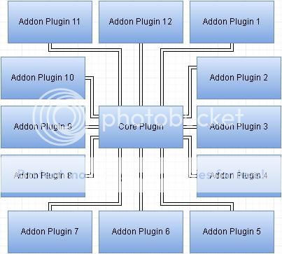
If we want to know the details of a plugin of a system, we can also use a block diagram for each plugin, which can be something like this:

Spoiler: ShowHide

If each feature's considered as a component, then this plugin's said to have 12 components(you may want to have a basic knowledge on interface in case you don't).


So as we go from a higher layer to a lower layer, more and more details of a component will be shown, but less and less information about how that component interact with the entire system as a whole will be revealed as well.
[/spoiler]
Showing Number Of Components

Spoiler: ShowHide

As mentioned, a system can have a number of plugins, a plugin can have a number of features, and a feature can have a number of building blocks. What levels of the details will be shown on a graph depends on the layer we're focusing on.


Sometimes though, the number of components within a system/plugin/feature can also be useful, like indicating whether a component's doing too much or too little.
Showcasing the number of components in a block diagram can be as simple as this:
[spoiler]

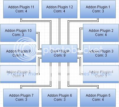
Here Com: x indicates the number of components within a plugin. In this case, it's the number of features within a plugin.
So the core plugin has 9 features and each addon plugin has 3 - 4 features. The total number of features of the whole system is 51.
From my experience, knowledge and observation, these are pretty good numbers, because it's normal for the core plugin to do a lot more than each addon plugin, and no plugin's doing too much or too little.


Note that a block diagram on a layer only shows the number of components on 1 lower layer for each component on this layer. It's because of the Law of Demeter.
In short, this approach ensures the overview shown by a high level block diagram won't be obscured by the details from lower levels, except the one just lower than the current level.
In this case, Com only shows the number of feature in each plugin, but not the number of building blocks of each feature in each plugin.
To know the number of building blocks of each feature in each plugin, we can look at the block diagram of that plugin instead.


On a side note: While the number of subcomponents within a component can be an excellent approximation of the size of that component in general, it's never meant to be always accurate nor precise for that sense. It's because sometimes a subcomponent can be exceptionally large or small.
[/spoiler]
[/spoiler]


Cohesion Diagram

Spoiler: ShowHide

Cohesion Rating(Coh Rating, Same Below)
[spoiler]
Let's recap different kinds of cohesion. According to wikipedia, the below are all kinds of cohesions that are ordered by the best to the worst:
1. Functional cohesion
2. Sequential cohesion
3. Communicational cohesion
4. Procedural cohesion
5. Temporal cohesion
6. Logical cohesion
7. Coincidental cohesion


If we were to use a number as a rating to represent the cohesion level of a component, we can simply use the above numbers - 1 represents functional cohesion, 2 represents sequential cohesion, 3 represents communicational cohesion, ..., 7 represents coincidental cohesion.
That's what's Coh Rating's about. The smaller the number, the higher the cohesion. Note that it's a simplified indicator that gives a quick, rouge and vague impression of how good the cohesion of a component is.

Showing Coh Rating Of A Component

Spoiler: ShowHide

Just like showing the number of components in a block diagram, showing the Coh Rating in a block diagram can be as simple as this:
[spoiler]

Here Coh: x indicates the Coh Rating of a plugin.
So the core plugin exhibits sequential cohesion and all addon plugins exhibit functional cohesion. The Coh Rating Sum of the whole system's 14.
From my experience, knowledge and observation, these are pretty good numbers, because functional cohesion's ideal and sequential cohesion's still acceptable.


Note that a block diagram on a layer only shows the Coh Rating of components on this layer. The reason behind that's basically the same as those of the number of components(Com: x).
In this case, Coh: x of a plugin only indicates the overall Coh Rating of that plugin, but not that of any feature within that plugin.


On a side note: The overall Coh Rating of the entire system can be different from that derived from diving its Cohesion Rating Sum(Coh Rating Sum, same below) by its number of components. Nevertheless, these 2 numbers are extremely unlikely to have a huge difference.
[/spoiler]
[/spoiler]


Coupling Digraph

Spoiler: ShowHide

Coupling Rating(Cou Rating, Same Below)
[spoiler]
Let's recap different kinds of coupling. According to wikipedia, the below are all kinds of couplings that are ordered by the best to the worst:
0. No coupling
1. Message coupling
2. Data coupling
3. Stamp coupling
4. Control coupling
5. External coupling
6. Common coupling
7. Content coupling


If we were to use a number as a rating to represent the coupling level of between components, we can simply use the above numbers - 1 represents message coupling, 2 represents data coupling, 3 represents stamp coupling, ..., 7 represents content coupling.
That's what's Cou Rating's about. The smaller the number, the looser the coupling. Note that it's a simplified indicator that gives a quick, rouge and vague impression of how good the coupling between components are.
On a side note: Temporal coupling's not included here, as it's rather hard to give a rating for temporal coupling, and the key of temporal coupling's how implicit it's. Making a temporal coupling explicit can be simply done by excellent documentations.

Showing Cou Rating Between Components

Spoiler: ShowHide

Showing the Cou Rating between components is a bit more complicated, convoluted and costly when compared to that of the number of components and Coh Rating, but it should still be easy, simple and small:
[spoiler]

Notice that this time arrows are used instead of merely simple lines, meaning that the block diagram's now a digraph.
If component A and component B are connected by an arrow which is pointing from component A to component B, then component A is said to depend on component B.
It's possible that they're connected by 2 arrows instead - 1 pointing from component A to component B and 1 having the opposite direction. In this case, these 2 components depend on each other.
Regardless of whether there are just 1 arrow or 2 arrows between these components, they're said to exhibit coupling when they're connected by at least 1 arrows.
Conversely, if component A and component B aren't connected by any arrows, they're said to exhibit no coupling.


Here Cou: x indicates the Cou Rating of a plugin. Note that a Cou Rating always has its corresponding arrow.
So the core plugin doesn't depend on any addon plugin while all addon plugins depend on the core plugin, all exhibiting message coupling/data coupling. The Coupling Rating Sum(Cou Rating Sum, same below) of the entire system's 18.
From my experience, knowledge and observation, these are pretty good numbers, because message coupling's ideal and data coupling's still acceptable and sometimes necessary.


Note that a block diagram on a layer only shows the Cou Rating between components on this layer. The reason behind that's basically the same as those of the number of components(Com: x) and Coh Rating(Coh: x).
In this case, Cou: x of a plugin only indicates the overall Cou Rating between plugins, but not that between features within any plugin or between plugins.


Bear in mind though, sometimes no coupling can be undesirable, as shown by the below block diagram:

Spoiler: ShowHide

Here addon plugin 4 exhibits no coupling to the rest of the system(i.e.:, the Cou Rating Sum of addon plugin 4 is 0), meaning that the former can function as intended without the latter at all.
In this case, addon plugin 4 doesn't really belong to the system and thus should be a completely separate plugin that can totally stand on its own instead.
[/spoiler]
InCou Rating/OutCou Rating

Spoiler: ShowHide

For components depending on each other, the block diagram may look something like this:
[spoiler]

If Cou: x is attached to an arrow directing from component A to component B, then the InCou Rating of component B from component A's x, and the OutCou Rating of component A to component B's x.
The InCou Rating Sum of a component's the sum of all InCou Rating of that component; The OutCou Rating Sum of a component's the sum of all OutCou Rating of that component.


Looking at each addon plugin:
1. For the InCou Rating of addon plugin 1, it exhibits message coupling from addon plugin 2 and data coupling from addon plugin 3; For the OutCou Rating of addon plugin 1, it exhibits It exhibits data coupling to core plugin and addon plugin 2, and message coupling to addon plugin 3.
2. For the InCou Rating of addon plugin 2, it exhibits message coupling from addon plugin 3 and data coupling from addon plugin 1; For OutCou Rating of addon plugin 2, it exhibits It exhibits data coupling to core plugin and addon plugin 3, and message coupling to addon plugin 1.
3. For the InCou Rating of addon plugin 3, it exhibits message coupling from addon plugin 1 and data coupling from addon plugin 2; For OutCou Rating of addon plugin 3, it exhibits It exhibits data coupling to core plugin and addon plugin 1, and message coupling to addon plugin 2.
Note that The InCou Rating Sum of each addon plugin's 3 and its OutCou Rating Sum's 5.
In this case, it's somehow undesirable although still barely bearable, as changing any addon plugin can risk changing the rest of the addon plugins. Ideally, each addon plugin should never interfere any other plugin, and only depend on the core plugin and nothing else.
On a side note: The Cou Rating Sum of the entire system's 15.


In general:
1. The larger the InCou Rating Sum of a component, the easier and more severely that component will be broken due to changes of any other component it's depending on.
2. The larger the OutCou Rating Sum of a component, the easier and more severely that component will break at least some other components depending on it due to it changes.
3. If a component has large InCou Rating Sum and OutCou Rating Sum, when it becomes broken due to changes of some components it depends on, it can in turn break some components depending on it.
[/spoiler]
[/spoiler]


Com Coh/Cou Digraph

Spoiler: ShowHide

Putting Everything Altogether
[spoiler]
While component diagram, cohesion diagram and coupling digraph are useful on their own, it's still better to combine them all in a single digraph. That's what Com Coh/Cou Digraph's about.
For example, combing all the above component diagram, cohesion diagram and coupling digraph can lead to this Com Coh/Cou Digraph:
[spoiler]

So a Com Coh/Cou Digraph can quickly shows the below information of its layer entirely:
1. The number of subcomponents of each component
2. The total number of subcomponents
3. The Coh Rating of each component
4. The Coh Rating Sum
5. The directed dependencies between components
6. The InCou Rating of each component
7. The OutCou Rating of each component
8. The InCou Rating Sum of each component
9. The OutCou Rating Sum of each component
10. The Cou Rating Sum of this layer


These information can reveal the overview of the structural health of a component corresponding to this Com Coh/Cou Digraph, which is useful for preliminary diagnosis, albeit without a 100% guarantee.
For instance, the above Com Coh/Cou Digraph demonstrates a pretty decent system design, because all its information shown is quite good.
On a side note: If drawing a Com Coh/Cou Digraph for a system's rather difficult, then it can mean that the system itself's incredibly ill-designed.
[/spoiler]
Relations Between Com, Coh, InCou And OutCou

Spoiler: ShowHide

The point of combining component diagram, cohesion diagram and coupling digraph into a single Com Coh/Cou Digraph isn't just to show all useful information in 1 shot, but also to demonstrate the relationships between those information.
For instance, the below Com Coh/Cou Digraph illustrates this:
[spoiler]

While it clearly and quickly demonstrates that the system has lots of structural health issues even when it seems to be easy, simple and small, let's still focus on each plugin 1 by 1:


1. Core plugin -
- As it exhibits communicational cohesion, which is generally considered to be a moderate code smell, the core plugin warrants detailed exploration, whether by using its own Com Coh/Cou Digraph or not.
- Compared to the total number of features of the whole system, which is 27, and the number of plugins in this system, which is 5, it's likely that the core plugin's still doing a bit too little.
- As the Coh Rating is a bit high when compared to the number of features, it can indicate that those features themselves are not well-defined enough, like some features overlapping too much with some others, or some features are simply wrapping up too many functionalities.


2. Addon plugin 1 -
- As it doesn't depend on the core plugin but rather another addon plugin, the depth of the system increases from 2 to 3, which complicates the system which is using the Core Addon Approach(the depth of such system should be always 2). It's because users must also activate another addon plugin in order to use this addon plugin.
- While it exhibits functional cohesion which is ideal, its number of components is also 1, meaning that this addon plugin's probably doing too little.
- As it exhibits content coupling with another plugin, which is generally considered to be 1 of the most destructive antipatterns, this plugin can break very easily and severely whenever addon plugin 4 changes. This can also lead to bugs that are actually due to this plugin even when they seem to stem from addon plugin 4.
- Combining all the above, it's likely that the entirety of this plugin should really be embedded as parts of addon plugin 4 instead, or the reverse - some features of addon plugin 4 should be placed on addon plugin 1, and the latter should depend on the core plugin instead of the former.


3. Addon plugin 2 -
- As it exhibits logical cohesion, which is generally considered to be a severe antipattern, it's likely that the features of this plugin doesn't really belong to the same plugin.
- As it only has 2 features while exhibiting logical cohesion, it's likely that the system designer isn't practicing system designs with excellent structural health. It's because normally the smaller number of components, the easier the cohesion to be higher.
- As it exhibits external coupling with another plugin, which is generally considered to be a moderate antipattern, it can mean that the features are probably not properly grouped or even well-defined, or addon plugin 4's simply an extremely ill-designed and implemented god object, especially when considering its high number of features, poor Coh Rating, and the high InCou Rating Sum.


4. Addon plugin 3 -
- As its number of features are 8 while it exhibits sequential cohesion which is still acceptable, this can either mean that those features are too small or the system's really covering a large number of features that are themselves tightly coupled, which can mean that those features are poorly defined.
- Nevertheless, it's probably the addon plugin with the best structural health.


5. Addon plugin 4 -
- It should be almost certain that this plugin's the one with the worst structural health, because it has the largest number of components which is clearly too large, the worst Coh Rating, the largest InCou Rating Sum and OutCou Rating Sum, and depends on and is depended on the largest number of plugins. It means that it's the addon plugin that should be dealt with first.
- It means that this addon's most likely an extremely ill-designed and implemented god object, which is already mentioned before.
- Combined with the fact that the core plugin's doing a bit too little, it's probable that some features of addon plugin 4 should belong to the core addon instead.
- Even then, addon plugin 4 will still likely be a big ball of mud, meaning that some of the rest of the features should be further delegated to some other existing of new addon plugins.
- Considering the fact that this plugin exhibits common coupling, which is generally considered to be a severe antipattern, with the core plugin, it seems that the this addon plugin affect so much of the system, as if it were the core plugin instead.
- Because of this plugin exhibiting control coupling, which is generally considered to be a severe code smell, to addon plugin 3, it looks like that the former's attempting to interfere with the latter. That's far from ideal in the Core Addon Approach, in which every addon plugin should never interfere with any other plugin, and only depend on and the core plugin and nothing else.


On a side note: The OutCou Rating Sum of the core addon should be 0, that of an addon plugin should be 1 or 2, and the InCou Rating Sum of an addon plugin should be 0.
[/spoiler]
[/spoiler]


Summary

Spoiler: ShowHide

Component Diagram
[spoiler]
For a layered system, a block diagram can demonstrate the structural overview of a component on a certain layer. When it's the highest layer, the block diagram can demonstrate the structural overview of the entire system. Such diagrams will only expose details on its layer and the one immediately below it, like the number of subcomponents in a component shown by the block diagram.
So as we go from a higher layer to a lower layer, more and more details of a component will be shown, but less and less information about how that component interact with the entire system as a whole will be revealed as well.
In short, this approach ensures the overview shown by a high level block diagram won't be obscured by the details from lower levels, except the one just lower than the current level.

Cohesion Diagram

Spoiler: ShowHide

A cohesion diagram can show the Coh Rating, which is a simplified indicator of how high the cohesion is, of a component in a block diagram, and the Coh Rating Sum of the diagram, which is the sum of Coh Rating of all components in the diagram. The lower the Coh Rating and Coh Rating Sum, the higher the cohesion in general.
The overall Coh Rating of the entire system can be different from that derived from diving its Coh Rating Sum by its number of components. Nevertheless, these 2 numbers are extremely unlikely to have a huge difference.

Coupling Digraph

Spoiler: ShowHide

A coupling digraph can show the Cou Rating, which is a simplified indicator of how loose the coupling is, between components in a digraph, and the Cou Rating Sum of the digraph, which is the sum of Cou Rating of all components in the diagram. The lower the Cou Rating and Cou Rating Sum, the looser the coupling in general.
The InCou Rating of a component indicates the coupling from other component to that component; The OutCou Rating of a component indicates the coupling from that component to other components.
The InCou Coupling Sum of a component is the sum of all InCou Rating of that component; The OutCou Coupling Sum of a component is the sum of all OutCou Rating of that component.
In general:
1. The larger the InCou Rating Sum of a component, the easier and more severely that component will be broken due to changes of any other component it's depending on.
2. The larger the OutCou Rating Sum of a component, the easier and more severely that component will break at least some other components depending on it due to it changes.
3. If a component has large InCou Rating Sum and OutCou Rating Sum, when it becomes broken due to changes of some components it depends on, it can in turn break some components depending on it.
For a component having 0 Cou Rating Sum, it means that component doesn't really belong to the system and should become a completely separate plugin that can totally stand on its own.

Com Coh/Cou Digraph

Spoiler: ShowHide

A Com Coh/Cou Digraph, which is a combination of a component diagram, cohesion diagram and coupling digraph, can reveal the overview of the structural health of its corresponding component, which is useful for preliminary diagnosis, albeit without a 100% guarantee. This is done by quickly showing all the useful information in 1 shot and demonstrating their relationships:
1. The number of subcomponents of each component
2. The total number of subcomponents
3. The Coh Rating of each component
4. The Coh Rating Sum
5. The directed dependencies between components
6. The InCou Rating of each component
7. The OutCou Rating of each component
8. The InCou Rating Sum of each component
9. The OutCou Rating Sum of each component
10. The Cou Rating Sum of this layer
For instance:
1. Normally the smaller number of components, the easier the cohesion to be higher.
2. Components having an exceptionally large/small number of subcomponents, having a poor Coh Rating, InCou Rating or OutCou Rating, or having an extraordinarily large InCou Rating Sum or OutCou Rating Sum, are most likely outstanding troublemakers and should thus be prioritized over those not as problematic.
If drawing a Com Coh/Cou Digraph for a system's rather difficult, then it can mean that the system itself's incredibly ill-designed.

[/spoiler]


That's all for now. As mentioned, I'll use some plugins to demonstrate some practical applications in the subsequent replies.